
# Welcome to my research page!
Below you can find some of the research topics that I’ve worked on in the past, am working on now, or would like to work on in the future! If you have any questions, feel free to reach out!
Contents
- Numerical relativity
- Gravitational wave memory
- Gravitational wave coordinate freedoms: the BMS group
- Binary black hole ringdowns
- Gravitational wave hybridizations
- Gravitational wave surrogate models
- Eccentric binary black hole models
- Active galactic nuclei (AGNs)
Numerical relativity
As one may imagine, while solving Einstein’s equations analytically for a single black hole is relatively simple (thanks Roy Kerr!), solving Einstein’s equations analytically for two black holes is effectively impossible and instead one solves them numerically by running a numerical simulation. A priori, however, Einstein’s equations aren’t set up in a form that’s easy to “evolve”. Consequently, to remedy this, we often write Einstein’s equations in what’s called “3+1 form”, i.e., specifying three spatial dimensions and one time dimension, with which we will evolve some space-like initial data. If one works in an appropriate gauge, i.e., a well-behaved coordinate system, then evolving this initial data becomes a well-posed problem (i.e., a solution will exist and be unique).
While this grossly oversimplifies the amount of work required to run a successful numerical relativity simulation, this is the main gist. And at the end of the day, if the code is written correctly, you can obtain some pretty remarkable simulations like this:
In the above simulation, color represents the lapse $\alpha$, which effectively describes how slow time flows due to the spacetime’s curvature. At the bottom there’s also a waveform representing the emitted gravitational wave, which is what we actually observe! But how do we compute that?
Earlier I mentioned that when simulating Einstein’s equations, it’s particularly important to understand and control the coordinate system that you’re using. And this is part of what makes numerical relativity so challenging: there’s an infinite number of coordinates to choose from! This is the general diffeomorphism invariance of general relativity. As a result, we can’t simply provide the LIGO-Virgo-KAGRA Collaboration with the spacetime metric on some worldline in our simulation because it would be highly dependent on the arbitrary coordinate system we chose. Instead, we need a way to limit how much we need to worry about coordinates. One way to do this is to look to some region of spacetime that has some kind of structure that we cannot simply change arbitrarily. But where to look? If we assume that the spacetime we’re simulating is asymptotically flat, i.e., that it has zero curvature infinitely far away from the origin, then we’ve naturally focused in on a region of spacetime with structure! While this boundary of spacetime can be partitioned into components, the one we will be interested in is called future null infinity—the final destination of outgoing null (i.e., light-like) radiation such as gravitational waves. Future null infinity, or $\mathcal{I}^{+}$ for short, has a particular structure that restricts what type of coordinate systems are valid. Furthermore, the metric takes on a particularly nice form known as the Bondi-Sachs metric:
\[\begin{align} ds^{2}&=-du^{2}-2dudr+2r^{2}\gamma_{z\bar{z}}dzd\bar{z}\nonumber\\ &\phantom{=.}+\frac{2m_{B}}{r}du^{2}+rC_{zz}dz^{2}+rC_{\bar{z}\bar{z}}d\bar{z}^{2}+D^{z}C_{zz}dudz+D^{\bar{z}}C_{\bar{z}\bar{z}}dud\bar{z}\nonumber\\ &\phantom{=.}+\frac{1}{r}(\frac{4}{3}(N_{z}+u\partial_{z}m_{B})-\frac{1}{4}D_{z}(C_{zz}C^{zz}))dudz+\mathrm{c.c.}+\cdots, \end{align}\]where “c.c.” stands for complex conjugation, $D_{z}$ is the covariant derivative with respect to the round metric on the two-sphere $\gamma_{z\bar{z}}$, $m_{B}$, $C_{zz}$, and $N_{z}$ are functions of $(u,z,\bar{z})$, and ellipsis represent subleading corrections. While “nice” may sound ironic after seeing the equation for the metric, it really is nice because $C_{zz}$ is exactly the gravitational wave that we observe in our gravitational wave detectors! So if we want to compute the gravitational wave in our simulations, then we simply need to solve Einstein’s equations in this Bondi-Sachs gauge.
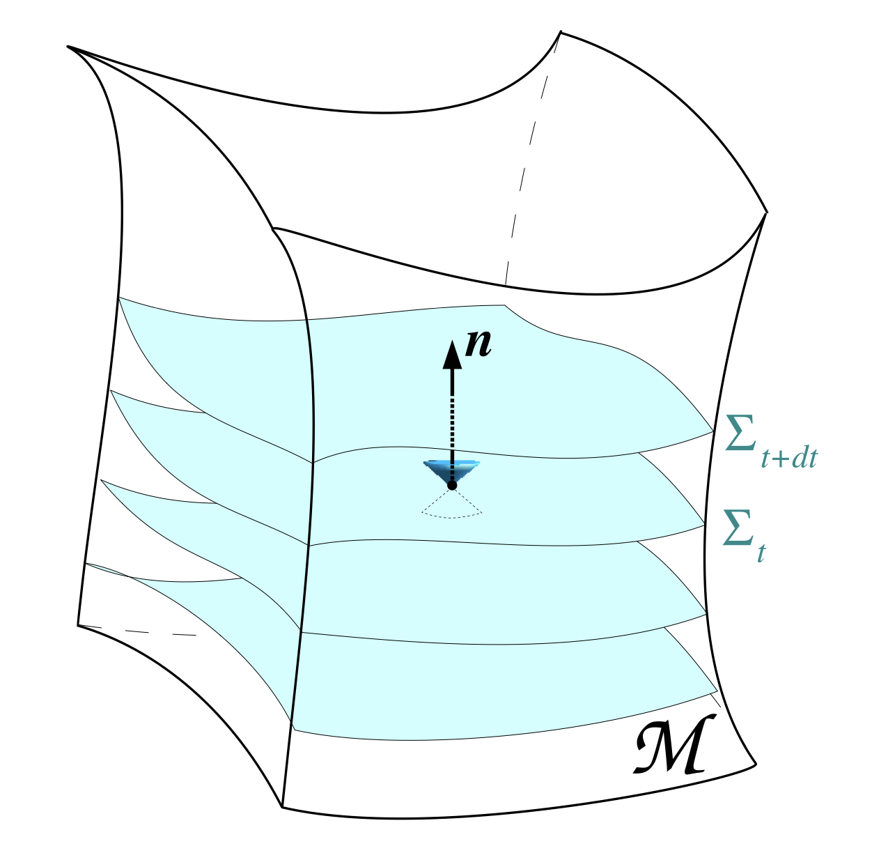
In practice this works via the following. First, solve Einstein’s equations for a gravitational system in 3+1 form on a series of Cauchy (i.e., space-like) slices, i.e., the blue foliations shown on the right. Then, at some radius, write the metric (and its derivatives) to file to produce a “worldtube” of metric data. Once this evolution is finished, one can then proceed to do a second evolution that includes future null infinity on the computational grid by compactifying the radial coordinate, i.e., redefining one’s coordinates so that instead of working with $r\in[r_{\mathrm{worldtube}},\infty]$ one works with finite coordinates, say, $y\equiv1-\frac{2r_{\mathrm{worldtube}}}{r}\in[-1,1]$.
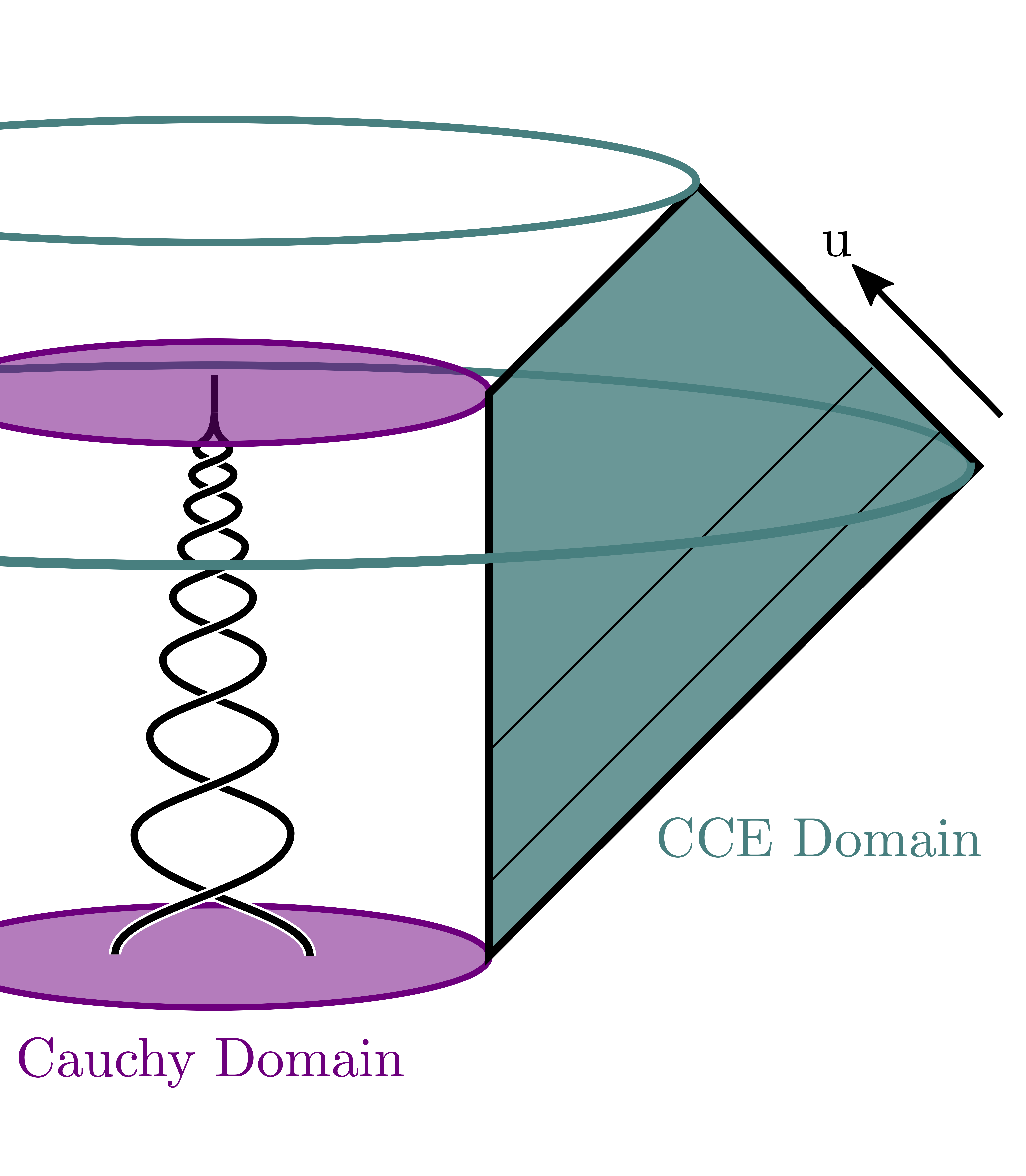
This evolution is called Cauchy-characteristic evolution (CCE), and instead evolves Einstein’s equations on null slices (rather than Cauchy slices). Furthermore, because the radial coordinate is compactified, future null infinity is included on the computational grid so one can easily compute the gravitational wave that current gravitational wave detectors observe! In fact, by performing a Cauchy evolution of a binary black hole coalescence that closely resembles the first gravitational wave detection, GW150914, using the SXS Collaboration’s code $\texttt{SpEC}$ followed by a Cauchy-characteristic evolution executed with the code $\texttt{SpECTRE}$, then one obtains the following solution to Einstein’s equations:
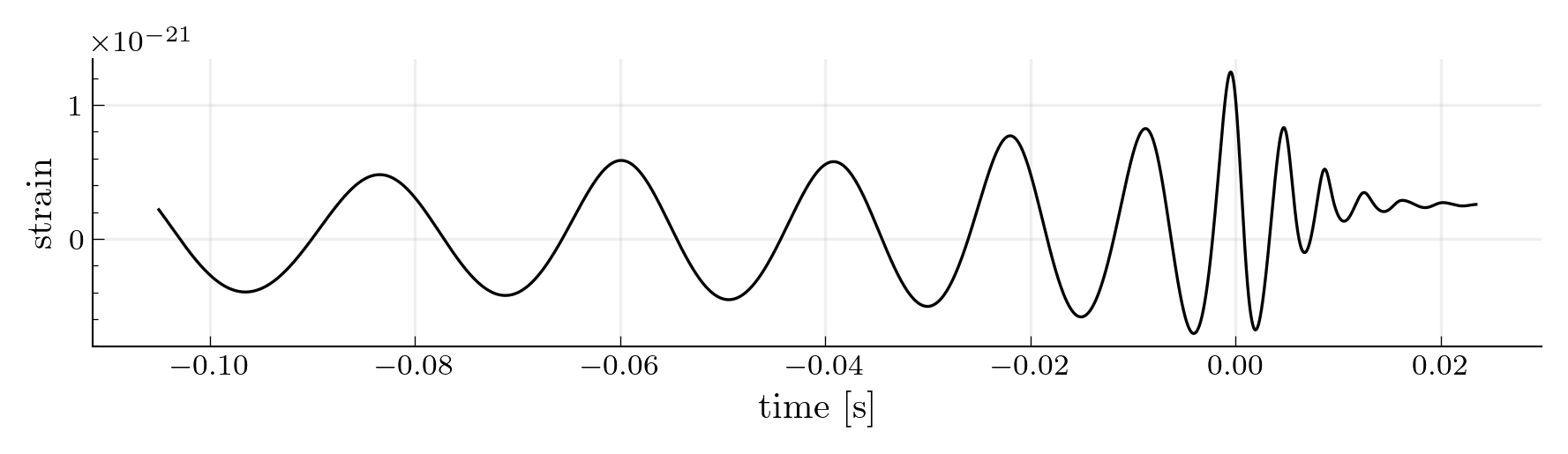
But what’s with the offset at the end? (hint: keep reading to find out)
Image Credit:
- SXS Collaboration, YouTube Channel
- Gourgoulhon, arXiv:gr-qc/0703035
- Moxon et al., arXiv:gr-qc/2110.08635
Gravitational wave memory
Above we saw that unlike what’s commonly presented in the literature, gravitational waves typically do not decay to zero at late times!
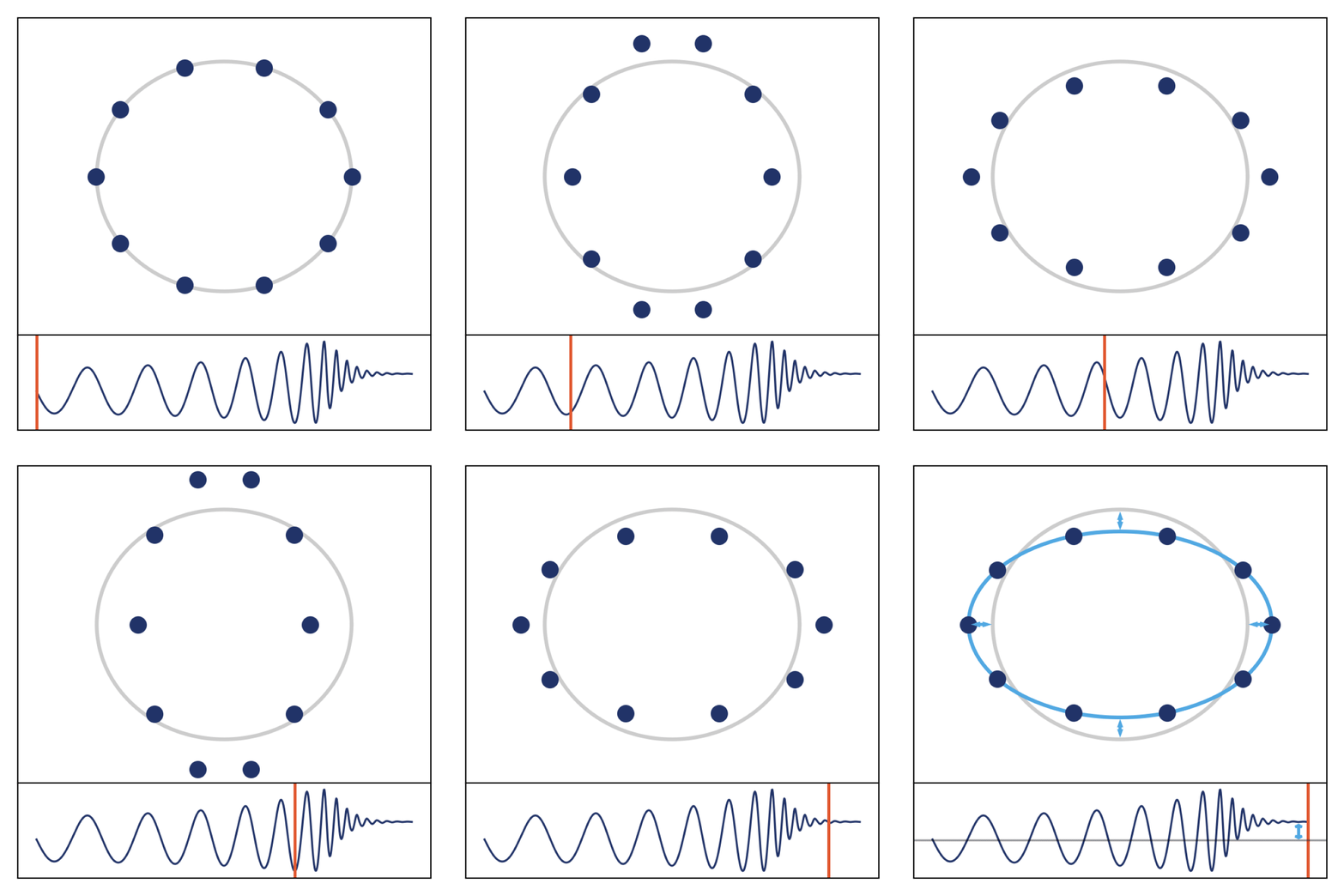
This phenomenon is known as the gravitational wave memory effect and corresponds to the fact that two freely-falling observers will experience a net displacement relative to each other due to a gravitational wave passing through the spacetime between them. This is illustrated through the GIF shown on the right. While time progresses, the spacetime between the observers (the points) oscillates with the peaks and the troughs of the gravitational wave. But, since the gravitational wave does not decay to zero at late times (due to the memory effect) the observers remain permanently displaced relative to their initial circular configuration! While this effect has yet to be observed, we can resolve it in numerical relativity simulations. And, in the next five-ish years, we expect to be able to claim a detection within the population of events observed by the LVK collaboration (see the last paragraph).
To do so, however, necessitates that one can separate out the memory contribution to the gravitational wave strain from the usual oscillatory contribution. So, in arXiv:2007.11562 and arXiv:2011.01309 (or see arXiv:2405.08868 for a review) we showed exactly how to do this with numerical relativity simulations! It turns out that because memory is intimately related to the symmetries of asymptotic infinity (see Gravitational wave coordinate freedoms: the BMS group) one can utilize Noether’s theorem to construct balance laws which naturally decompose the strain into a component which looks like the usual oscillatory contribution and a component which looks like the step-like memory contribution. Consequently, understanding whether or not we’ve observed memory in a gravitational wave observation is trivial (provided that we can observe a binary black hole coalescence with a high enough signal-to-noise ratio!)
In arXiv:2605.27500, we used hierarchical Bayesian inference to combine the binary black hole observations in the LVK’s GWTC-5.0 catalog and search for the memory. We constrained the “memory enhancement factor”—the term in front of the step-like memory contribution to the strain—which equals one in general relativity and zero when memory is absent, to $0.26_{-4.08}^{+4.09}$. Therefore, the present observations are consistent with general relativity, but are not yet precise enough to distinguish its prediction from no memory at all. Even so, we found that roughly 2,000 detections will be needed to make this distinction at the $1\sigma$ level, which should happen with O6; stay tuned!
Gravitational wave coordinate freedoms: the BMS group
In Numerical Relativity we explained why it is much easier to study gravitational radiation from gravitational systems at future null infinity. In particular, the added structure of the boundary of asymptotically flat spacetimes makes it so that the coordinate freedoms one must control are not arbitrary diffeomorphisms, but rather a more restricted set of symmetries. While one may naively expect the symmetries of future null infinity to simply be the 10 Poincaré symmetries—four spacetime translations, three Lorentz rotations, and three Lorentz boosts—it turns out that there is actually an infinite number of symmetries, which are contained in a particular extension of the Poincaré group known as the BMS group, named after Bondi, van der Burg, Metzner, and Sachs.
These additional symmetries of the BMS group come from the fact that future null infinity is built from an infinite number of null generators: one for each point on the celestial two-sphere (mathematically we have $I^{+}\cong\mathbb{R}\times S^{2}$). Physically, a way to think of this is the following. Imagine you have a group of observers watching some event, say a supernova. If these observers know their relative positions, then they can change their personal clocks so that they all receive the same spherically-symmetric information at the same time. However, if you push these observers to asymptotic infinity, then they become causally disconnected from one another, so there is no way for them to synchronize their personal clocks to begin with, meaning these “direction-dependent” time translations, a.k.a., “supertranslations”, are a symmetry of the system.
Consequently, whenever one computes a gravitational waveform at future null infinity, it is subject to the infinite number of BMS freedoms, which must be controlled in some well-defined manner! Across arXiv:2105.02300 and arXiv:2208.04356 (with a review in arXiv:2405.08868), we describe exactly how this can be done to compare NR waveforms from different resolutions, or NR waveforms to other waveform approximants, like post-Newtonian waveforms! (see below!)
Binary black hole ringdowns
Immediately after two black holes merge, the remnant is not born as a perfectly stationary Kerr black hole. Instead, it is highly distorted and sheds those distortions by emitting a superposition of damped oscillations known as quasinormal modes (QNMs). Much like the tones of a struck bell, each QNM has a characteristic frequency and decay time. For a Kerr black hole these quantities are determined entirely by the remnant’s mass and spin (the so-called “no-hair theorem”), so measuring more than one tone allows us to perform “black hole spectroscopy” and test whether the remnant really behaves as predicted by general relativity.
Before we can compare a numerical relativity ringdown to black hole perturbation theory, however, we have to make sure that both waveforms are written in the same coordinates. A QNM calculation naturally assumes a frame adapted to the final Kerr black hole: the remnant superrest frame. Numerical waveforms are generally rotated, boosted, and even supertranslated relative to this canonical BMS frame—as discussed in Gravitational wave coordinate freedoms: the BMS group! Both arXiv:2110.15922 and arXiv:2208.04356 showed how to map numerical waveforms into the remnant superrest frame. Doing so can improve QNM identification and help find new physics!
In particular, it turns out that a ringdown is richer than a sum of only the longest-lived linear modes. In arXiv:2208.07380, we showed that second-order, or nonlinear, QNMs are necessary to accurately describe the ringdown’s higher harmonics. In particular, the dominant $(2,2)$ mode can couple to itself and produce a quadratic contribution to the $(4,4)$ harmonic. The amplitude of this nonlinear tone scales as the square of its parent mode and can be as large as, or even larger than, the ordinary linear $(4,4)$ mode!
The early ringdown also contains overtones: QNMs with the same angular structure as the fundamental tone, but which decay more quickly. Because they disappear so rapidly, it can be difficult to determine whether an apparent overtone is a real physical excitation or merely a flexible fit to the complicated waveform near merger. In arXiv:2411.11269 and arXiv:2503.09678, we developed stability tests and a systematic extraction procedure that confirm multiple overtones across high-accuracy numerical relativity simulations. Surprisingly, these tones allow black hole perturbation theory to describe the waveform remarkably close to the waveform’s peak!
Most recently, these ideas became directly relevant for the extraordinarily clear signal GW250114. In arXiv:2509.08099, the LVK Collaboration found that the signal’s post-merger data require at least two tones: the dominant $(2,2)$ fundamental mode and its first overtone. Furthremore, a full inspiral-merger-ringdown analysis managed to constrain the $(4,4)$ fundamental QNM, and all of the measured frequencies and decay times were consistent with a Kerr black hole. The animation above first shows the binary’s inspiral and merger phases, and then separates the remnant’s fundamental tone, first overtone, and the predicted third tone constrained by the observation. Consequently, GW250114 provides a spectacular demonstration that the detailed ringdown physics we study in simulations can now be tested using real gravitational wave data!
Image Credit:
- Harald Pfeiffer, LIGO Lab
Gravitational wave hybridizations
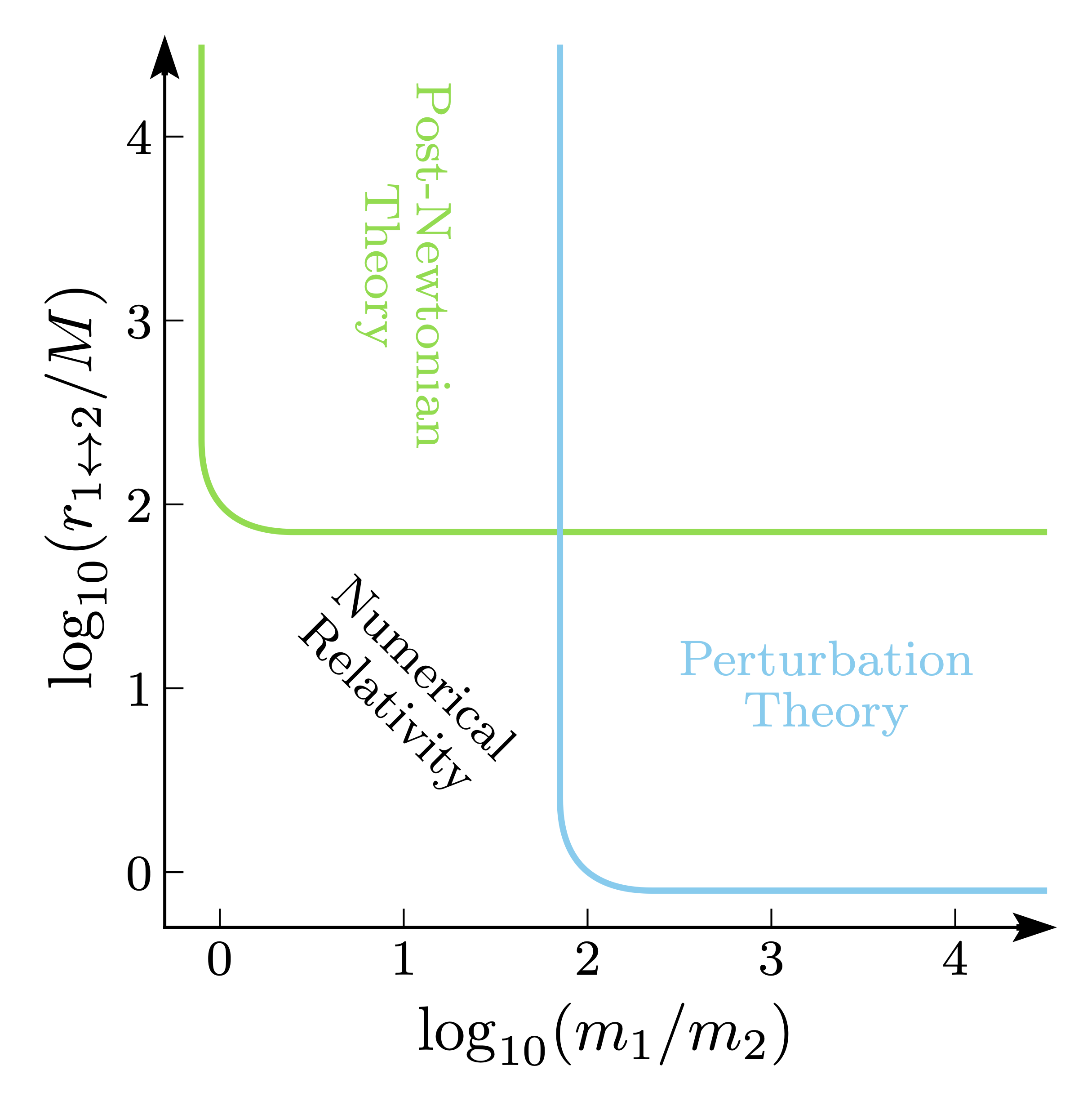
As may be obvious, running long NR simulations is challenging because they require more compute time. Furthermore, simulating binaries with large mass ratios, e.g., $q\gtrsim20$, is also challenging since a large number of spatial points are needed to capture the dynamics around the smaller body. So, if we want to build waveforms that span low frequencies and all mass ratios (both of which are desperately needed for many of the next-generation detectors!) we need some alternative to NR, or at least some way to extend NR to these regimes. This is where hybrids come in handy!
For now we’ll focus on how to extend NR waveforms to cover lower frequencies (the problem of building “hybrids” to extend to higher mass ratios is more a “hybrid” in the NR simulation, rather than a post-processing hybrid. See arXiv:2410.22290 for more details!). As can be seen in the diagram to the upper right, while NR isn’t really practical for binary separations $\gtrsim100M$, this is where post-Newtonian (PN) theory shines.
Post-Newtonian theory works by assuming that the characteristic velocities of the bodies sourcing the radiated gravitational wave are slow compared to the speed of light, i.e., $(v/c)^2\sim GM/rc^2\ll1$. This assumption is useful because when one writes Einstein’s equations in their “relaxed” form in harmonic gauge, i.e., $\square h^{\alpha\beta}=-16\pi(G/c^4)\tau^{\alpha\beta}$ for $\square\equiv-\partial^2/\partial (ct)^2+\nabla^2$ and $\tau^{\alpha\beta}$ the effective energy-momentum pseudotensor, one has $h^{\alpha\beta}(t,\mathbf{r})$ via: \begin{align} h^{\alpha\beta}(t,\mathbf{r})=\frac{4G}{c^4}\int\frac{\tau^{\alpha\beta}(t-|\mathbf{r}-\mathbf{r’}|/c,\mathbf{r’})}{|\mathbf{r}-\mathbf{r}’|}d^{3}r’, \end{align} which readily yields the usual quadrupole formula for our slow motion limit (see Wald section 4.4)! Furthermore, one can push to higher orders in the perturbation expansion, i.e., higher orders in the small parameter $(v/c)^2$, to obtain more and more accurate predictions. Consequently, one can use PN to approximate the gravitational wave strain when the binary is well-seperated, and then switch to NR once the dynamics become more complex. However, there are a few caveats that arise when doing this “switch”, i.e., when constructing the PN-NR hybrid waveform.
For one, PN predictions and NR waveforms are typically in completely different BMS frames (see Gravitational wave coordinate freedoms: the BMS group)! So before a hybrid can be constructed, NR has to be mapped to the frame of PN, which we effectively solved in arXiv:2105.02300 and arXiv:2208.04356. A more annoying issue, however, is that the definition of the black hole progenitor parameters in PN and NR also need not be the same! In PN, the mass and spin are effectively defined in the infinite past. However, in NR, they are defined quasi-locally from each black holes apparent horizon; hence they mean something different than those of PN. To account for this, it turns out that one needs to optimize for the PN parameters that best match NR (while also optimizing over the BMS frame). In arXiv:2403.10278 we explored this for the first time and found that performing both of these optimizations indeed yields ideal PN-NR hybrid waveforms.
Gravitational wave surrogate models
As discussed above, numerical relativity provides us with our most accurate predictions for the gravitational waves emitted during the coalescence of two black holes. Unfortunately, an individual numerical relativity simulation can take days to months to complete on a supercomputer, while analyzing a gravitational wave observation requires comparing the observed signal to thousands, or even hundreds of thousands, of waveforms. So running new simulations every single time that the LVK Collaboration asks “what binary could have produced this signal?” isn’t much of an option!
This is where surrogate models come to the rescue. The basic idea is to begin with a collection of expensive, high-accuracy waveforms and use them to identify a much smaller set of basis waveforms that captures nearly all of the relevant behavior. One then determines the times at which the waveform contains the most useful information, fits how that information changes throughout the 9-dimensional binary parameter space (or some subset of it), and combines these pieces to rapidly reconstruct the waveform at a new point. The animation below provides a wonderful visual overview of this entire procedure.
Once trained, a surrogate can compute a waveform for a point in parameter space in tens of milliseconds while closely reproducing the much more expensive simulations on which it was built. In this sense, a surrogate is a carefully constructed emulator of an entire family of simulations, which is fast enough for preforming parameter estimation and tests of general relativity.
Much of my work on surrogate modeling has focused on making sure that the training waveforms contain all of the physics that we want the model to reproduce. In arXiv:2306.03148, for example, we constructed the $\texttt{NRHybSur3dq8_CCE}$ model from CCE waveforms that were mapped into a common BMS frame and hybridized with post-Newtonian and effective-one-body waveforms. Unlike earlier waveform models, this surrogate successfully captures the gravitational wave memory effect discussed above and predicts waveforms in the same frame as PN.
Many numerical relativity surrogate models are distributed through the public $\texttt{GWSurrogate}$ package described in arXiv:2504.08839. Consequently, surrogate modeling provides a bridge between the accuracy of simulations and the speed required by gravitational wave astronomy. And, as numerical-relativity catalogs grow to include more extreme mass ratios, spins, and eccentricities, surrogate models provide a direct way to turn those expensive calculations into tools that can be used on extract meaningful science from real world observations!
Image Credit:
- Vijay Varma, Surrogate modeling
Eccentric binary black hole models
Nearly all of the black hole systems discussed above are assumed to be on quasicircular orbits. This is often a good approximation because gravitational waves carry away orbital energy and angular momentum in a manner that tends to strongly circularize the binary before it enters into the LVK’s frequency band. But binaries assembled by dynamical encounters in dense environments, or influenced by a third nearby object, can merge before completely circularizing. If so, their gravitational waves contain bursts near each pericenter passage and characteristic modulations in both amplitude and frequency. These features make the waveforms more complicated, but they also provide valuable clues about how the binary formed!
Modeling eccentric binaries, however, is substantially harder than modeling quasicircular ones. Besides the masses and spins, one must keep track of both the eccentricity and the binary’s location within its radial cycle, usually described by the mean anomaly. These extra dynamics affect not only the inspiral waveform, but also the properties of the remnant black hole left behind. In arXiv:2605.00124, we constructed two numerical-relativity surrogate models for nonspinning eccentric binaries: one predicts the final black hole’s mass, spin, and recoil velocity, while the other tracks the time evolution of the eccentricity and mean anomaly. Among other applications, these models show how eccentricity can either enhance or suppress the remnant’s recoil depending on where the binary is in its orbit when it merges, which matters for active galactic nuclei simulations!
Ultimately, accurate and fast eccentric models will allow us to search for these systems without forcing their signals into a quasicircular description. And if we can reliably measure even a small residual eccentricity, gravitational waves can tell us not only what merged, but also something about where and how the binary was assembled!
Image Credit:
- Harald Pfeiffer, animation associated with arXiv:2302.11257
Active galactic nuclei (AGNs)
I’ve been working with the McFACTS team to integrate surrogate models into their code; look out for a paper and a description of the physics we learned soon!